时间序列语言模型：预测分析的新范式_AI阅读总结 — 包阅AI

It’s no secret that the rise of large language models (LLMs) like ChatGPT and Bard has dramatically changed how many work, communicate, and learn. But LLMs have applications other than replacing search engines. Most recently, data scientists have repurposed LLMs for time series forecasting.

Time series data is ubiquitous across domains, from financial markets to climate science. Meanwhile, powered by advancements in artificial intelligence, LLMs are revolutionizing the way we process and generate human language. Here, we dive into how time series LMs provide innovative forecasting and anomaly detection models.

What Is a Time Series LM?

At a high level, time series LMs are repurposed to handle time series data rather than text, video, or image data. They combine the strengths of traditional time series analysis methods with the advanced capabilities of LMs to make predictions. Strong forecasts can be used to detect anomalies when data deviates significantly from the predicted or expected result. Some other notable differences between time series LMs and traditional LLMs include:

• Data Type and Training: While traditional LLMs like ChatGPT are trained on text data, time series LMs are trained on sequential numerical data. Specifically, pre-training is performed on large, diverse time series datasets (both real-world and synthetic), which enables the model to generalize well across different domains and applications.
• Tokenization: Time series LMs break down data into patches instead of text tokens (a patch refers to a contiguous segment, chunk, or window of the time-series data).
• Output Generation: Time series LMs generate sequences of future data points rather than words or sentences.
• Architectural Adjustments: Time series LMs incorporate specific design choices to handle the temporal nature of time-series data, such as variable context and horizon lengths.

Time series language models (LMs) offer several significant benefits over traditional methods for analyzing and predicting time series data. Unlike conventional approaches, such as ARIMA, which often require extensive domain expertise and manual tuning, time series LMs leverage advanced machine learning techniques to learn from the data automatically. This makes them robust and versatile tools for many applications where traditional models might fall short.

Zero-shot performance: Time series LMs can make accurate predictions on new, unseen datasets without requiring additional training or fine-tuning. This is particularly useful for rapidly changing environments where new data emerges frequently. A zero-shot approach means users don’t have to spend extensive resources or time training their model.

Complex pattern handling: Time series LMs can capture complex, non-linear relationships and patterns in data that traditional statistical models like ARIMA or GARCH might miss, especially for data that hasn’t been seen or preprocessed. Additionally, tuning statistical models can be tricky and require deep domain expertise.

Efficiency: Time series LMs process data in parallel. This significantly speeds up training and inference times compared to traditional models, which often process data sequentially. Additionally, they can predict longer sequences of future data points in a single step, reducing the number of iterative steps needed.

Time Series LMs in Action

Some of the most popular time series LMs for forecasting and predictive analytics include Google’s TimesFM, IBM’s TinyTimeMixer, and AutoLab’s MOMENT.

Google’s TimesFM is probably the easiest to use. Install it with pip, initialize the model, and load a checkpoint. You can then perform a forecast on input arrays or Pandas DataFrames. For example:

Google’s TimesFM also supports fine-tuning and covariate support, which refers to the model’s ability to incorporate and utilize additional explanatory variables (covariates) alongside the primary time series data to improve the accuracy and robustness of its predictions. You can learn more about how Google’s TimesFM works in this paper.

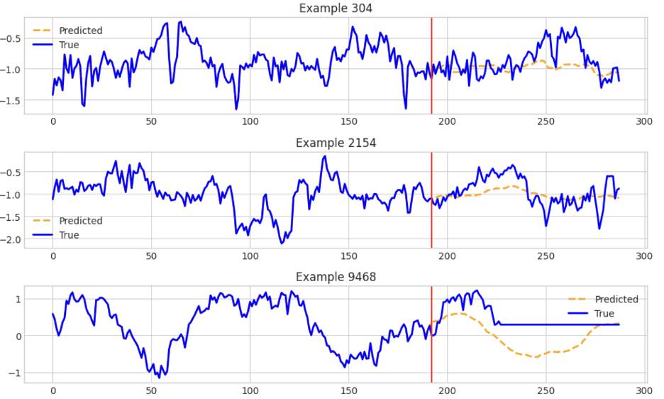
IBM’s TinyTimeMixer contains models and examples for performing various forecasts on multivariate time series data. This notebook highlights how to use the TTM (TinyTimMixer) to perform both zero-shot and few-shot forecasts on data. The screenshot below shows some of the estimates that TTM produced:

Finally, AutoLab’s MOMENT has methods of forecasting and anomaly detection with easy-to-follow examples. It specializes in long-horizon forecasting. As an example, this notebook highlights how to forecast univariate time series data by first importing the model:

The next step is training the model on your data for proper initialization. After each training epoch, the model is evaluated on the test dataset. Within the evaluation loop, the model makes predictions with the line output = model(timeseries, input_mask).

Final thoughts

Time series LMs represent a significant advancement in predictive analytics. They marry the power of deep learning with the intricate demands of time series forecasting. Their ability to perform zero-shot learning, incorporate covariate support, and efficiently process large volumes of data positions them as a transformative tool across various industries. As we witness rapid progress in this area, the potential applications and benefits of time series LMs will only expand.

To store time series data, check out InfluxDB Cloud 3.0, the leading time series database. You can leverage the InfluxDB v3 Python Client Library with InfluxDB to store and query your time series data and apply a time series LLM for forecasting and anomaly detection. You can check out the following resources to get started: