
包阅导读总结
1. 关键词:Vector Database、HNSW、Pgvector、Approximate Nearest-Neighbor Search、Indexing
2. 总结:本文主要介绍了向量数据库中 HNSW 索引,包括其在 Pgvector 中的应用、与其他索引方法的比较、工作原理、创建步骤等,强调其对高效管理高维数据和适应动态数据集的优势。
3. 主要内容:
– Vector Database Basics
– 介绍向量数据库及向量在其中的作用
– Pgvector and HNSW Indexes
– Pgvector 支持 HNSW 索引用于高维向量数据的快速近似近邻搜索
– HNSW 索引的优势在于无需扫描整个数据集
– Approximate Nearest-Neighbor Search (ANN)
– 是计算问题,可在搜索精度和计算效率间权衡
– 分为树、哈希、图三类,HNSW 利用图结构处理高维数据
– HNSW vs IVF
– HNSW 适应动态数据集,管理插入和删除无需重建索引
– 对比 IVF 索引的局限性
– How Does HNSW Work?
– 原理:利用图结构组织数据,最小化点间路径长度
– 受跳表启发,构建多层图
– 引入长边缘,克服传统图索引挑战
– How to Create HNSW?
– 包括构建分层结构、图构建和实际实现方面的步骤
思维导图: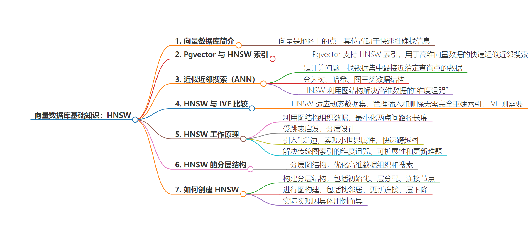
文章地址:https://www.timescale.com/blog/vector-database-basics-hnsw/
文章来源:timescale.com
作者:Team Timescale
发布时间:2024/8/13 15:10
语言:英文
总字数:2605字
预计阅读时间:11分钟
评分:88分
标签:向量数据库,HNSW 索引,近似最近邻搜索,pgvector,TimescaleDB
以下为原文内容
本内容来源于用户推荐转载,旨在分享知识与观点,如有侵权请联系删除 联系邮箱 media@ilingban.com
When it comes to machine learning and AI systems, vector databases are essential tools for storing and searching through vast amounts of data. Imagine vectors as points on a map, where each point has its unique location. In the context of databases, these “locations” help us find the information we need quickly and accurately.
Pgvector is an extension for PostgreSQL that allows the storage and retrieval of vector data in the database. It supports HNSW (hierarchical navigable small world) indexes, which enable fast approximate nearest-neighbor searches for high-dimensional vector data. HNSW indexes are essential because they efficiently find similar vectors without scanning the entire dataset. This is valuable when working with large amounts of high-dimensional vector data, where scanning all vectors becomes slow.
The primary goal of this article is to explain HNSW indexes, highlighting why they’re better than older methods and how to use them with pgvector. We’ve tailored this guide for anyone who works with vector databases, develops AI applications, or is curious about modern data search. We’ll also touch on how this technology is integrated with TimescaleDB and show how it enhances data management capabilities at scale for real-life applications.
The HNSW Index on Pgvector
Pgvector’s introduction of the hierarchical navigable small world index is an excellent addition to its ability to manage vector databases efficiently. This methodology, originating from the foundational work by Malkov and Yashunin, breaks new ground in the domain of approximate nearest-neighbor search (ANN) by offering a novel, graph-based framework.
This framework is especially crucial for high-dimensional data, where traditional indexing struggles to maintain efficiency due to the exponential increase in complexity brought on by each added dimension.
Exploring approximate nearest-neighbor search (ANN)
Approximate nearest-neighbor search (ANN) is a computational problem that focuses on finding data points in a dataset closest to a given query point. Unlike exact nearest-neighbor search, ANN allows for a trade-off between search accuracy and computational efficiency, acknowledging that exact matches can be prohibitively expensive regarding computation time and resources in high-dimensional spaces.
ANN can be divided into three primary categories, each defined by its foundational data structures: trees, hashes, and graphs. Trees hierarchically organize data, allowing for binary decisions at each node to navigate closer to the query point. Hashes convert data points into codes in a lower-dimensional space, grouping similar items into the same buckets for faster retrieval.
Graphs, which HNSW utilizes, create a network of points where edges connect neighbors based on similarity measures. Among these, HNSW stands out for its use of a multi-layered graph structure that efficiently tackles the “curse of dimensionality”—an issue that impacts high-dimensional data spaces by making traditional search methodologies inefficient and often infeasible.
HNSW’s layered graph approach enables it to approximate searches rather than striving for exact matches, significantly reducing computational overhead without substantially compromising accuracy.
This method acknowledges the inherent limitations in handling high-dimensional data, emphasizing practicality and performance over perfection. It cleverly navigates the data space by progressively narrowing the search area across its hierarchical layers, ensuring that searches remain fast and relevant.
Distinguishing HNSW from IVF
When comparing HNSW with the inverted file (IVF) indexing approach, one of HNSW’s standout features is its adaptability to dynamic datasets—it efficiently manages inserts and deletes without necessitating a complete rebuild of the index. This dynamic nature is pivotal for continuously evolving applications, requiring the index to be as fluid as the data it represents.While powerful in their usage, IVF indexes often need to be entirely reconstructed to accommodate new data or remove old, which can be time-consuming and hinder real-time search capabilities. HNSW’s design circumvents this limitation, offering a more sustainable solution for databases where change is constant.
How Does HNSW Work?
Understanding how the HNSW algorithm works requires a closer look at its principles, its inspiration from skip lists, and how it introduces long edges to overcome traditional graph indexing challenges.
Principles of HNSW
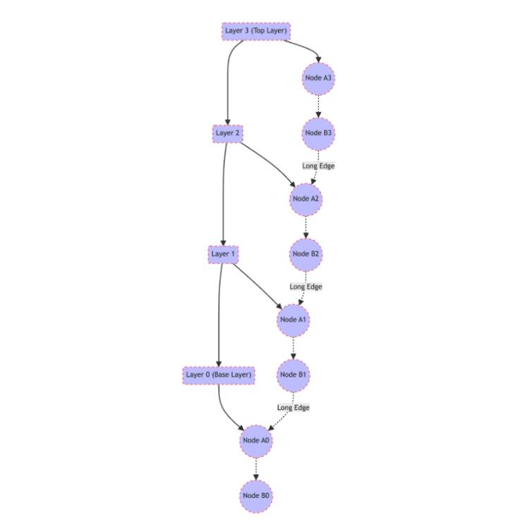
HNSW leverages a graph structure to organize data in a way that reflects the inherent similarities between data points, forming a navigable small world network. The principle guiding this structure is to minimize the path length between any two points in the graph, ensuring that each point is reachable from any other through a small number of hops. This is achieved by organizing the data into multiple layers, with each successive layer offering a more refined view of the data.
Inspiration from skip lists
Skip lists, a data structure for storing a sorted list of items with efficient search, insertion, and deletion operations, inspire HNSW’s hierarchical design. In a skip list, elements are organized into layers, with higher layers providing shortcuts for quickly traversing the list.
Similarly, HNSW constructs multiple layers of graphs, where the top layers contain fewer nodes and serve as highways for rapid navigation across the data space, directing searches closer to the target before diving into denser, lower layers for fine-grained search.
Introducing “long” edges
In the context of HNSW, “long” edges refer to connections in the upper layers of the graph that span large distances in the data space, bypassing many intermediate nodes. These edges are critical for achieving the small-world property, allowing quick jumps across the graph.
As a search query moves down from the top layer to the bottom, the length of the edges decreases, and the search area becomes increasingly localized, enabling precise identification of the nearest neighbors with minimal computational overhead.
Addressing traditional graph indexing challenges
Traditional graph indexing techniques often struggle with the curse of dimensionality, where the distance between data points becomes less meaningful in high-dimensional spaces. This makes it challenging to organize and search the data efficiently. They also suffer from poor scalability and difficulty updating the index as new data points are added or removed.
HNSW addresses these issues through its multi-layered, hierarchical approach. It allows for efficient search by reducing the dimensionality at each layer and dynamically adjusting the graph’s structure without needing complete rebuilds.
This design improves search efficiency in high-dimensional spaces and supports incremental updates, making HNSW particularly well-suited for dynamic datasets where data points frequently change.
In summary, HNSW’s optimized approach to organizing and searching high-dimensional data leverages the principles of navigable small-world networks and skip lists, introducing long edges to facilitate rapid navigation. This structure significantly overcomes the limitations of traditional graph indexing techniques, offering a scalable, dynamic, and efficient solution for approximate nearest-neighbor search.
How to Create HNSW?
Creating an HNSW index involves several steps, focusing on building the hierarchical structure, constructing the graph with its multi-layered approach, and the practical aspects of implementation.
Building the hierarchical structure
The hierarchical structure of HNSW is fundamentally a set of layered graphs, each representing the dataset with varying degrees of abstraction. The top layer has the fewest nodes and serves as the entry point for search queries, facilitating rapid traversal across the data space. Each subsequent layer increases in density, adding more detail until reaching the base layer, which contains all data points.
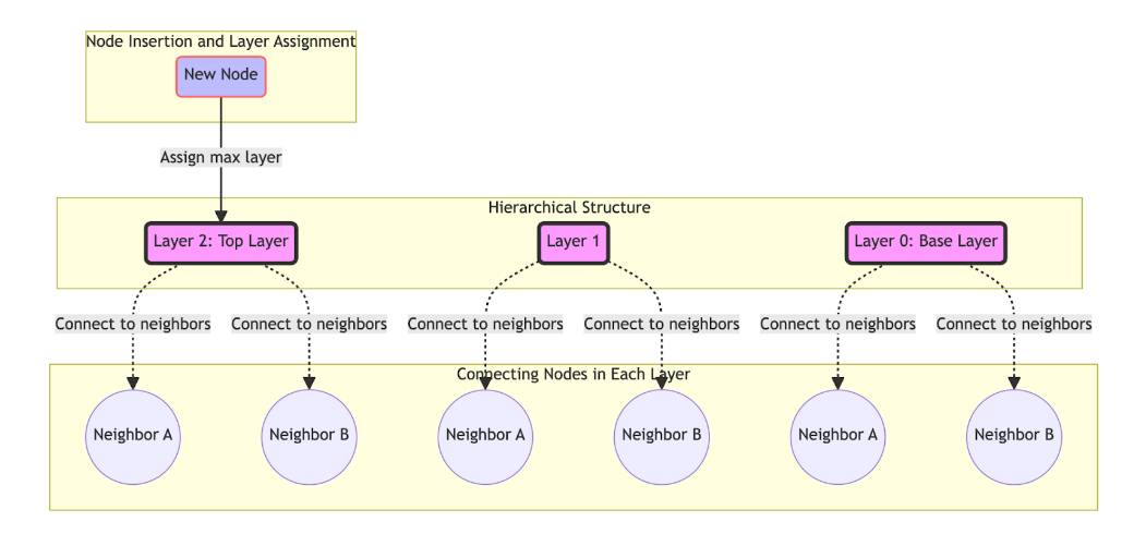
- Initialization: Start with an empty structure. The graph has no nodes initially, and the first inserted node becomes the sole member of the top layer.
- Layer assignment: For each new data point, determine its maximum layer, l, within the hierarchy. This is typically done using a probabilistic method, such as flipping a coin or drawing from a geometric distribution, to ensure that the expected number of nodes decreases as the layer height increases.
- Connecting nodes: Insert the new node into each layer to its assigned maximum layer. In each layer, connect the node to its closest neighbors. The number of connections, or edges, a node has in each layer can be fixed or variable, influenced by parameters like the desired level of sparsity or density for the graph.
Graph construction
Graph construction populates the hierarchical structure with data points and establishes connections based on similarity or proximity.
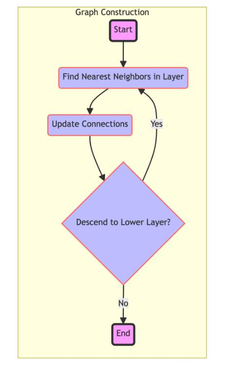
- Finding neighbors: Identify the nearest neighbors of an inserted new node in the current layer. This can involve searching the entire graph or using heuristics to limit the search space. Initially, the search starts from a randomly selected node or a designated entry point updated as the graph grows.
- Updating connections: Once the nearest neighbors in a layer are identified, the new node’s connections are established. This may require updating the neighbors’ connections to ensure the graph remains navigable and that the small-world property is preserved.
- Layer descent: Repeat the process for each layer below the node’s maximum layer, refining the search for nearest neighbors as the graph becomes denser. This iterative approach ensures that each node is optimally placed within the hierarchical structure, maintaining efficient navigability.
Implementation
The practical implementation of HNSW can vary based on specific use cases and performance requirements. However, some common considerations include:
- Language and library choices: Implementations can be created in various programming languages. C++ is often chosen for its balance between high-level usability and low-level control over memory and performance. Libraries like nmslib or faiss provide optimized distance calculations and graph operations routines.
- Memory management: Efficient memory usage is critical, especially for large datasets. This involves choosing appropriate data structures for storing nodes and edges and managing the hierarchical layers.
- Parallelization: To speed up the construction and query processes, HNSW implementations can leverage parallel computing techniques. This includes parallelizing the search for nearest neighbors and the insertion of nodes, as well as managing concurrency issues that may arise.
In implementing HNSW, attention to detail in these areas can significantly impact the performance and scalability of the index, making it suitable for a wide range of applications in search and data retrieval in high-dimensional spaces.
The HNSW Approach: Merits and Challenges
The HNSW indexing algorithm brings several advantages and challenges. Understanding these can help effectively leverage HNSW for vector database management and search applications.
Merits
- Well documented: One of HNSW’s significant advantages is its strong documentation and the wealth of research backing its methodology. This robust foundation aids developers and researchers in understanding, implementing, and optimizing the algorithm for various applications.
- Preferred index in vector databases: HNSW has become the index of choice across numerous vector database engines. Its efficiency in high-dimensional vector space search operations makes it highly sought after for applications in AI, machine learning, and similar domains where rapid retrieval of information based on vector similarity is crucial.
- Configurability for high recall and speed: HNSW offers exceptional configurability, allowing it to be tuned for high recall—the ability to retrieve the most relevant results—without significantly compromising search speed. This balance is particularly valuable in scenarios where the accuracy of search results is paramount, and results need to be obtained quickly.
Challenges
- Memory-intensive: HNSW’s performance relies heavily on storing the index entirely in memory. While beneficial for speed, this architecture choice makes HNSW more suitable for systems with substantial RAM availability. The memory requirement can become a limiting factor as the dataset grows, especially into the tens of millions of high-dimensional vectors.
- Scales with memory, not disk: Unlike other data storage and indexing methods that efficiently utilize disk space, HNSW’s design necessitates that the entire index fit within the available memory. This characteristic can pose challenges in scaling the system for extensive datasets or in environments where memory resources are constrained.
Creating HNSW Indexes in Pgvector
Integrating HNSW into your projects for efficient vector search capabilities can be surprisingly straightforward, especially with tools like AI and vector on Timescale Cloud and its support in SQL and Python environments.
With Timescale Cloud, developers can access pgvector, pgvectorscale, and pgai—extensions that turn PostgreSQL into an easy-to-use and high-performance vector database, plus a fully managed cloud database experience.
Here’s how to leverage HNSW with a single line of code in each context, making your vector database more powerful and search-efficient, whether in our cloud platform or using the open-source version.
Creating an HNSW index in SQL with pgvector on Timescale
TimescaleDB, an extension of PostgreSQL designed to handle time-series data, events, and analytics, also extends its functionality to support vector operations through pgvector. Implementing HNSW indexing for your vector data stored in a PostgreSQL database can significantly enhance search performance.
Here’s how you can create an HNSW index on a table’s embedding column in SQL:
CREATE INDEX document_embedding_idx ON document_embedding USING hnsw(embedding vector_cosine_ops);This command creates an HNSW index named document_embedding_idx for the document_embedding table on the embedding column using cosine similarity operations (vector_cosine_ops). This index facilitates efficient nearest-neighbor searches using the HNSW algorithm’s speed and accuracy.
Utilizing HNSW in Python With Timescale Library
For those working within a Python environment, the Timescale Python library simplifies applying HNSW indexing to your vector data.
Here’s how to create an HNSW index using the library:
vec.create_embedding_index(client.HNSWIndex()) This line of code instructs the library to create an HNSW index on the vector data managed by the vec object.
For more control over the indexing process, including tuning the algorithm’s parameters for even better performance, you can specify additional options like this:
vec.create_embedding_index(client.HNSWIndex(m=16, ef_construction=64, ef_search=10))This extended example sets the m, ef_construction, and ef_search parameters to customize the HNSW index. Here, m controls the maximum number of connections for each element in the index, ef_construction adjusts the size of the dynamic list used during index construction for better accuracy, and ef_search influences the search time precision.
Overcoming HNSW Limitations
While HNSW is the preferred index in vector databases, its memory-intensive nature can be a hurdle for developers working with large datasets. This is where pgvectorscale stands out, delivering high performance without eating away at your disk space and memory.
By adding a StreamingDiskANN index to pgvector, pgvectorscale overcomes the limitations of in-memory indexes—like HNSW. It stores part of the index on disk, making it more cost-efficient to run and scale as vector workloads grow. This vastly decreases the cost of storing and searching over large amounts of vectors since SSDs are much cheaper than RAM.
Pgvectorscale also supports streaming filtering, which allows for accurate retrieval even when secondary filters are applied during similarity search. It adds statistical binary quantization (SBQ) to pgvector, improving accuracy over traditional methods of quantization.
The result is increased search performance at higher accuracy from indexes that take up less space on disk and in memory. And all at a quarter of the cost of specialized databases, like Pinecone.
The combination of pgai—which brings AI workflows into PostgreSQL—with pgvectorscale and pgvector enables developers to keep using the PostgreSQL they know and love by turning it into a high-performance platform for vector workloads and building AI applications. See how you can get started today.
Conclusion
Throughout this article, we’ve explored HNSW indexing, enhancing the efficiency and accuracy of ANNS in high-dimensional data spaces. Starting with its operational principles, we’ve seen how HNSW stands out for its performance and flexibility.
By breaking down the process of constructing an HNSW index and highlighting its strengths and limitations, we aimed to provide a comprehensive understanding of its impact on vector database management. The HNSW index offers a compelling blend of speed, precision, and ease of use, making it the index of choice for many applications in AI, machine learning, and beyond.
Despite its memory-intensive nature and challenges in scaling large datasets, HNSW’s benefits in facilitating rapid and accurate searches are undeniable. For those ready to integrate HNSW into their projects, whether through SQL commands or the Python-based Timescale library, the process is straightforward yet powerful. With just a line of code, you can unlock the potential of your vector data, enhancing your applications’ search capabilities.
Working with scaling datasets? Install the pgvectorscale PostgreSQL extension and start building more scalable AI applications with higher-performance embedding search and cost-efficient storage.
Ingest and query in milliseconds, even at terabyte scale.