
包阅导读总结
1. 关键词:火箭控制系统、控制理论、Python、PID 控制器、稳定性分析
2. 总结:本文主要介绍如何运用控制理论和 Python 构建火箭控制系统,包括控制理论的作用、火箭控制系统的类比、创建步骤、PID 控制器的原理和关键部分,以及稳定性分析和代码示例。
3. 主要内容:
– 控制理论与火箭控制系统
– 控制理论是研究使系统按期望方式运行的学科
– 火箭控制系统是复杂系统,本文基于火箭探讨控制理论的应用
– 火箭控制系统的类比
– 以烤蛋糕为例,说明火箭、飞行计划和控制行动的关系
– 控制系统的重要性及应用领域
– 有助于算法设计和系统思考
– 应用于机器人、信号处理、嵌入式系统等领域
– 创建火箭控制系统的步骤
– 选择控制策略
– 建立数学模型
– 设置初始参数
– 调整测试
– 优化参数
– 实现设计
– 火箭控制中的 PID 控制器
– 介绍 PID 控制器的工作原理
– 包括比例增益、积分增益和微分增益的作用
– 稳定性分析
– 介绍根轨迹、波特图和奈奎斯特图用于稳定性分析
– 转移函数与组件值
– 阐述理论和物理转移函数的作用
– 说明如何确定物理转移函数方程
– 代码示例
– 导入相关库
– 定义火箭转移函数
– 设计 PID 控制器
– 应用 PID 控制器
– 绘制根轨迹、波特图和奈奎斯特图
思维导图: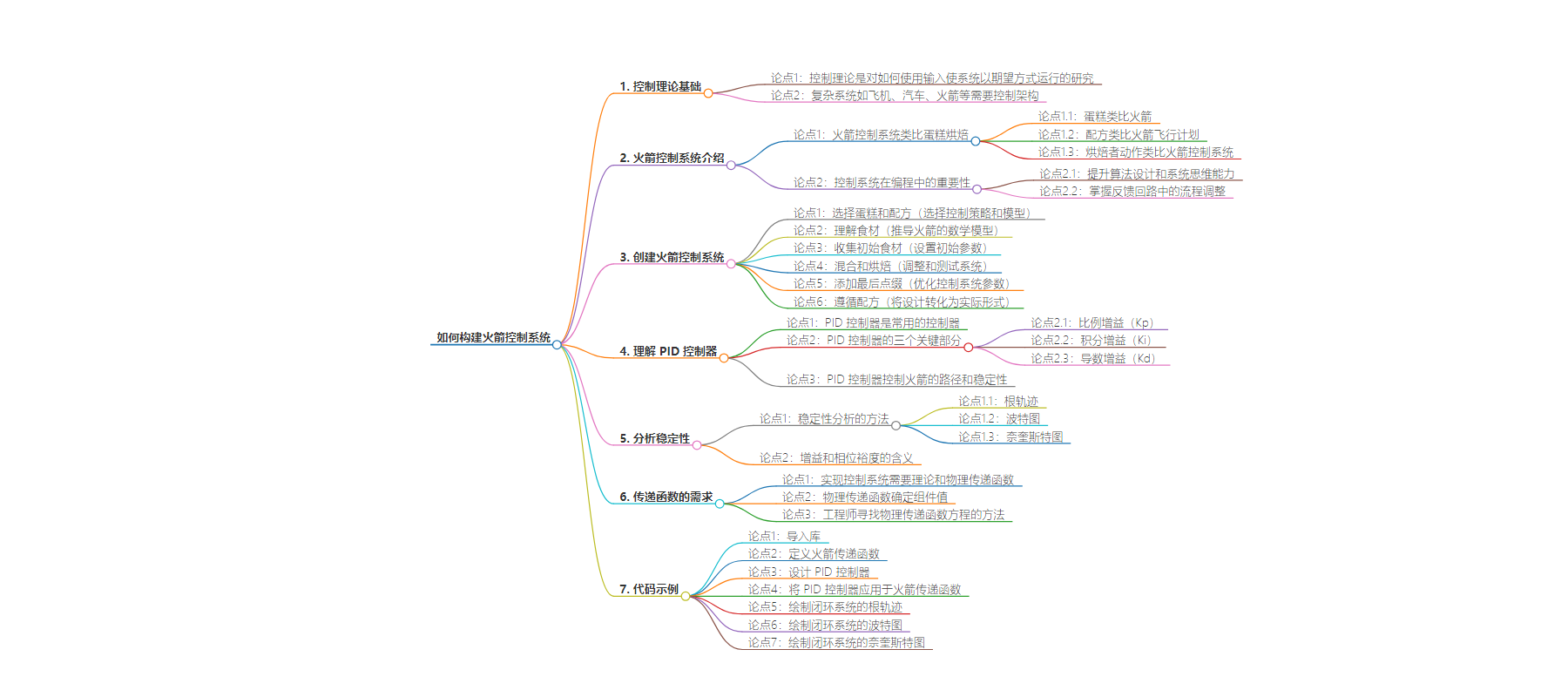
文章地址:https://www.freecodecamp.org/news/basic-control-theory-with-python/
文章来源:freecodecamp.org
作者:Tiago Monteiro
发布时间:2024/8/6 14:26
语言:英文
总字数:2680字
预计阅读时间:11分钟
评分:86分
标签:控制系统,Python 编程,PID 控制器,火箭工程,稳定性分析
以下为原文内容
本内容来源于用户推荐转载,旨在分享知识与观点,如有侵权请联系删除 联系邮箱 media@ilingban.com
Building any control systems, including a rocket control system, involves combining control theory with programming.
Control theory is the study of how to make systems behave in a desired way using inputs.
Planes, cars, trains, circuits, rockets and many more systems need to have a brain or an architecture inside them.
Control theory is the study of the control architectures of these complex systems.
In this article, we will explore how to apply control theory to create a rocket control system using Python.
This is a simple guide to how the architecture of complex systems is created. In this case, it’s based on a rocket.
In this article, you will learn about:
Note: We’ll assume the rocket is time-invariant, meaning its behavior doesn’t change over time. Addressing time-varying dynamics would complicate this tutorial more than I’d like.
Rocket Systems and Cake Baking: A Fun Comparison
 Photo by Brent Keane on Pexels
What is a Rocket Control System?
Imagine you are backing a cake. Your recipe provides the steps and ingredients needed to bake the cake.
In this analogy:
- The cake is the rocket
- The recipe is the rocket flight plan
- The baker’s actions are the rocket control system
Just as you change the oven temperature or mixing time to get the best cake, a control system changes rocket’s parameters to ensure it stays on its course and remains stable.
Why are control systems important in programming?
By understanding control systems, you’ll become better at algorithmic design and systems thinking.
It also enables you to figure out how to adjust processes in feedback loops. This is very important in many areas of programming.
You’ll mainly use control theory and control systems when creating software for:
- Robotics and Automation: Control systems enable precise movement and adaptability in robots using feedback loops based on sensor input.
- Signal Processing and Communication: They optimize data transmission, error correction, and filtering for reliable communication.
- Embedded Systems and IoT: Control systems manage device interactions with environments, processing sensor inputs and adjusting outputs efficiently.
How to Create a Rocket Control System
In terms of our cake baking analogy:
- Choose the Cake and Recipe: Select a simple control strategy, like choosing a basic cake recipe. A common choice is a PID controller because it’s simple and effective.
- Understanding the Ingredients: Derive a mathematical model of the characteristics and trajectory of the rocket. Like studying the recipe and ingredients. This way, we get a clear understanding of the system.
- Gathering Initial Ingredients: Set initial parameters, similar to gathering your basic ingredients.
- Mixing and Baking: Adjust and test the system, much like mixing ingredients and baking. This involves using various graphs to check stability and performance.
- Adding Final Touches: Fine-tune the parameters, just like adding final decorations to your cake, to optimize the control system for efficiency.
- Following the Recipe: Convert your design into a practical form, like carefully following a cake recipe.
Rocket Control Made Simple: Understanding PID Controllers
A simple control system: The PID controller
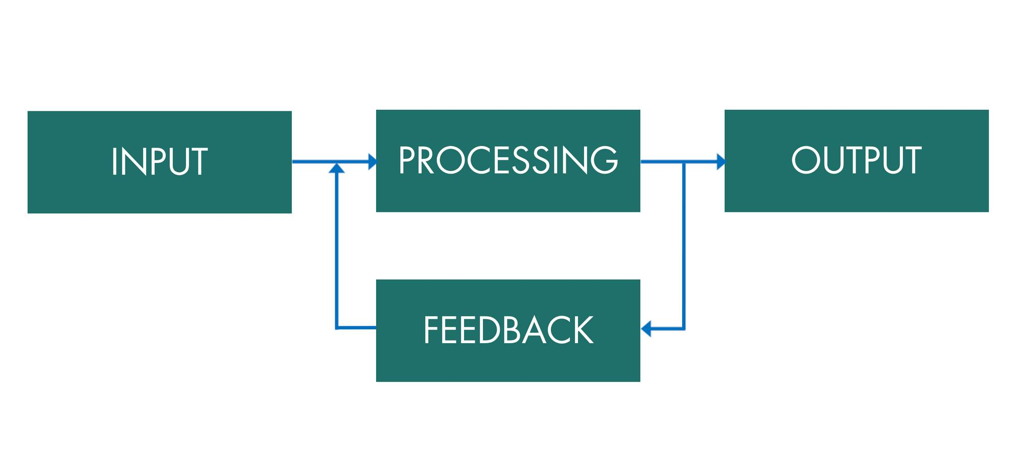 Example of control system diagram (source)
Every control system has a controller that runs it. One of the most used controllers is the PID controller.
In the code example here, we will use the PID controller. This is because it’s simple and effective for simple control systems.
In a rocket control system, the rocket’s PID controller constantly adjusts the rocket’s path (processing block) by comparing its current position to where it should be (feedback block).
This way, the rocket stays on course and reaches its final destination.
The PID controller has three key parts that work in the processing and feedback part of the system: proportional gain (Kp), integral gain (Ki), and derivative gain (Kd).
- The proportional gain (Kp): Reacts immediately to any error, making the system respond quickly but sometimes causing it to overshoot the target.
- The integral gain (Ki): Fixes past errors by adding them up over time, getting rid of any leftover errors, but it can make the system unstable if set too high.
- The derivative gain (Kd): Predicts future errors to help prevent overshooting and smooth out the system’s response.
This is why it’s called a PID (Proportional-Integral-Derivative) controller.
These three parts work together to create a control signal that changes the rocket’s setting. This ensures that it’s stable, accurate and effective.
With the PID controller, we can control how the inputs like thrust and altitude change the position and speed to ensure the rocket is stable and on its intended path.
Analyzing Stability
 Photo by Shiva Smyth on Pexels
To design a PID controller means to design a stable control system.
The process of designing a stable control system is called stability analysis.
There are many methods, but in the code example we will use:
- Root locus: Shows system stability and response
- Bode plot: Displays system gain and phase margins
- Nyquist plot: Illustrates stability and potential oscillations
In this case, the gain and phase margins simply mean that the control system can tolerate changes.
The gain margin tells us how much the system gain can increase without losing stability. Gain means how much to amplify the input signal to make the output signal.
The phase margin tells us how much delay is tolerable without losing stability. Delay in control theory means how much time it takes for the output to respond to the input.
This tells us how to change the Kp, Ki, and Kd so that the PID controller can control the rocket in an effective manner.
The Need for Transfer Functions: Controlling the Rocket and Determining Component Values
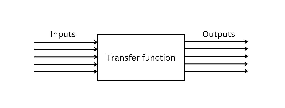
To implement any control system, we need two transfer functions: one theoretical and one physical.
Transfer functions tell us how inputs convert to outputs in a mathematical way.
The theoretical function is, in this case, the PID controller.
The physical system transfer function represents real-world dynamics and behavior of the physical components in the system.
By combining both, we can understand the behavior of materials and component values such as:
- Capacitor values for energy storage
- Sensor calibration values for accurate data measurement and feedback
- Spring constants for shock absorption systems
- Pressure ratings for fuel and oxidizer tanks
This way, the PID controller is not only the brain of the rocket but also can tell us the values of the components needed so that the rocket can fly its path.
How do engineers find the physical transfer function equation?
First, we need to understand what the rocket is for.
Will it send a LEO (Low Earth Orbit) or MEO (medium Earth orbit) satellite to space or a rocket to the moon?
After knowing its use case, we can, with math and physics, find the physical equation of the transfer function.
There is actually an entire field of engineering called system identification dedicated to this.
Now let’s see how to find, for any control system, its physical transfer function.
Code example: Designing a simple PID controller
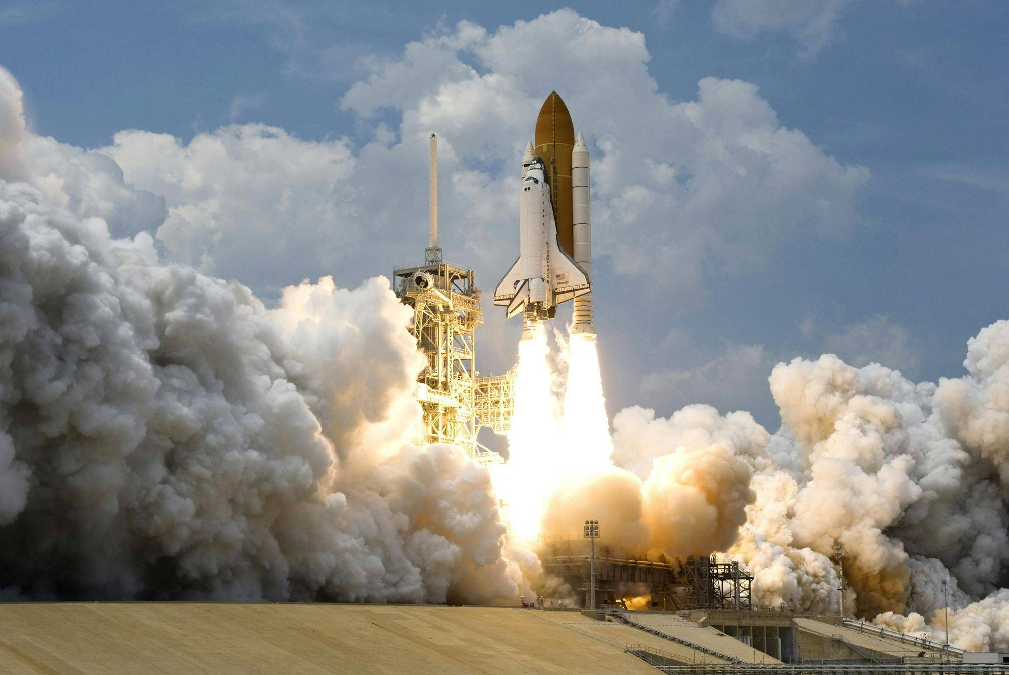 Photo by Pixabay
Now with this code example, we will create a simple control system for a rocket.
Before we dive into the code, let’s talk about decibels.
Decibels use a logarithmic scale to measure sound. In control theory, they measure gain in a way that’s easier to visualize on graphs.
This way, we can see many more large and small values in a manageable range.
In other words, by seeing the gain in a logarithmic scale, we are seeing how much the input is amplified to be the output in a manageable range of values.
I’ll also explain how root locus, Bode plot, and Nyquist plots assist engineers in stability analysis.
Let’s see the code – and then we’ll analyze it block by block:
# Step 1: Import librariesimport matplotlib.pyplot as pltimport control as ctrl# Step 2: Define a new rocket transfer function with poles closer to the imaginary axisnum = [10] den = [2, 2, 1] G = ctrl.TransferFunction(num, den)# Step 3: Design a PID controller with new parametersKp = 5Ki = 2Kd = 1C = ctrl.TransferFunction([Kd, Kp, Ki], [1, 0])# Step 4: Applying the PID controller to the rocket transfer functionCL = ctrl.feedback(C * G, 1)# Step 5: Plot Root Locus for Closed-Loop Systemplt.figure(figsize=(10, 6))ctrl.root_locus(C * G, grid=True)plt.title("Root Locus Plot (Closed-Loop)")# Step 6: Plot Bode Plot for Closed-Loop Systemplt.figure(figsize=(10, 6))ctrl.bode_plot(CL, dB=True, Hz=False, deg=True)plt.suptitle("Bode Plot (Closed-Loop)", fontsize=16)# Step 7: Plot Nyquist Plot for Closed-Loop Systemplt.figure(figsize=(10, 6))ctrl.nyquist_plot(CL)plt.title("Nyquist Plot (Closed-Loop)")plt.show()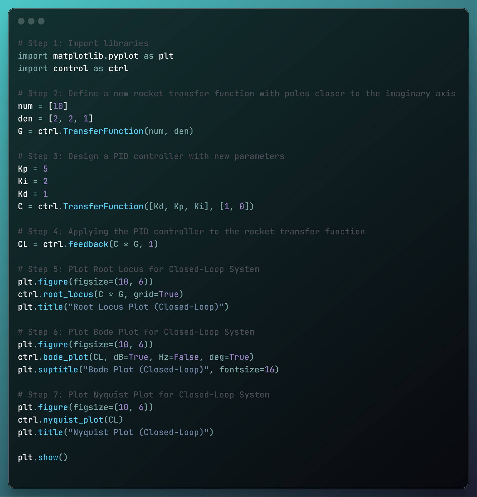 Full Code
Step 1: Import libraries
import matplotlib.pyplot as pltimport control as ctrl Importing libraries
Here we import two libraries:
- matplotlib: A plotting library for creating various types of visualizations
- Control: A library for analyzing and designing control systems
Step 2: Define the Transfer Function of the Rocket System
num = [10] den = [2, 2, 1] G = ctrl.TransferFunction(num, den)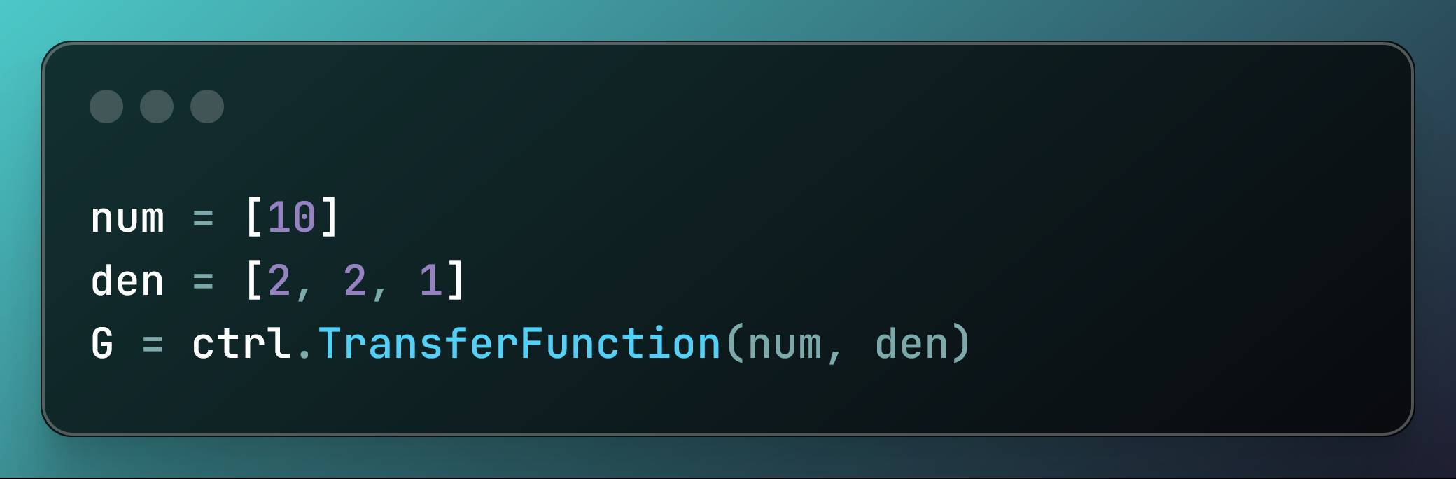 Define the Transfer Function of the Rocket System
In this code we define the transfer function of the physical system
num=[10]: Sets the system gain to 10.den=[2,2,1]: Defines the denominator.G = ctrl.transferFunction(num, cen): Constructs the transfer function.
This is the transfer function we are going to control with PID:
<!DOCTYPE html>
Black-Scholes Equation
$$\frac{\partial V}{\partial t} + \frac{1}{2}\sigma^2 S^2 \frac{\partial^2 V}{\partial S^2} = rV – rS \frac{\partial V}{\partial S}$$
Rocket transfer function
In this code example, the transfer function rocket equation is very simple. But in real life, rocket transfer functions are not time-invariant linear systems. Usually, they are very complex non-linear systems.
Step 3: Design a PID controller with new parameters
Kp = 5Ki = 2Kd = 1C = ctrl.TransferFunction([Kd, Kp, Ki], [1, 0])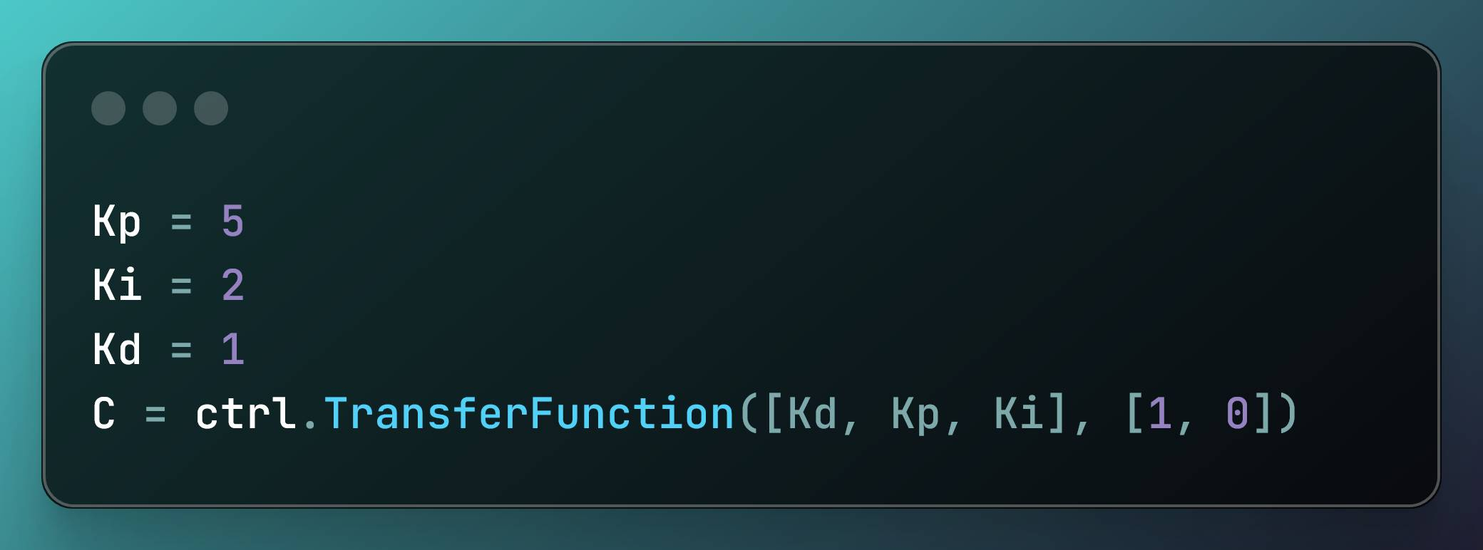 Design a PID controller with new parameters
This code sets up a PID controller with specific gains and creates a transfer function:
Kp = 5: Sets the proportional gain to 5.Ki = 2: Sets the integral gain to 2.Kd = 1: Sets the derivative gain to 1.C = ctrl.TransferFunction([Kd, Kp, Ki], [1, 0]): Creates a transfer function of the PID controller
Step 4: Applying the PID controller to the rocket transfer function
CL = ctrl.feedback(C * G, 1)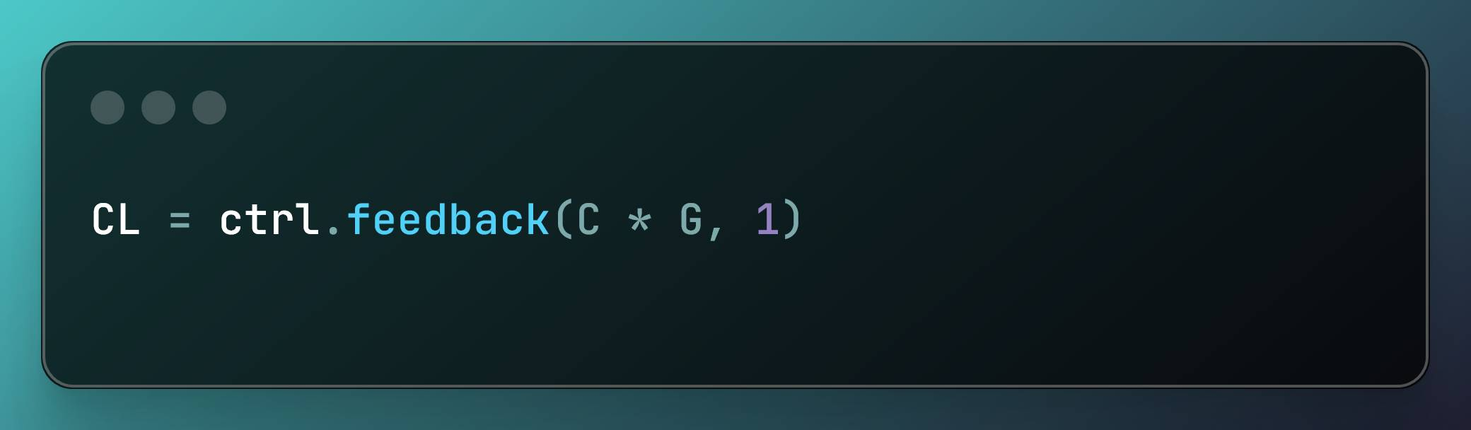 Applying the PID controller to the rocket transfer function
C * G: Multiplies the PID controllerCwith the systemG(the rocket) to form the open-loop transfer function, which models the system’s behavior without feedback and relies on predefined settings.ctrl.feedback(C * G, 1): Computes the closed-loop transfer function by applying feedback and representing the system’s behavior with feedback. This allows it to adjust inputs and automatically correct errors.CL: Stores the resulting closed-loop system, integrating the controller with the rocket to maintain desired performance through feedback, and is used for further analysis or simulation.
Step 5: Root Locus for gain analysis
In this code:
plt.figure(figsize=(10, 6))ctrl.root_locus(C * G, grid=True)plt.title("Root Locus Plot (Closed-Loop)")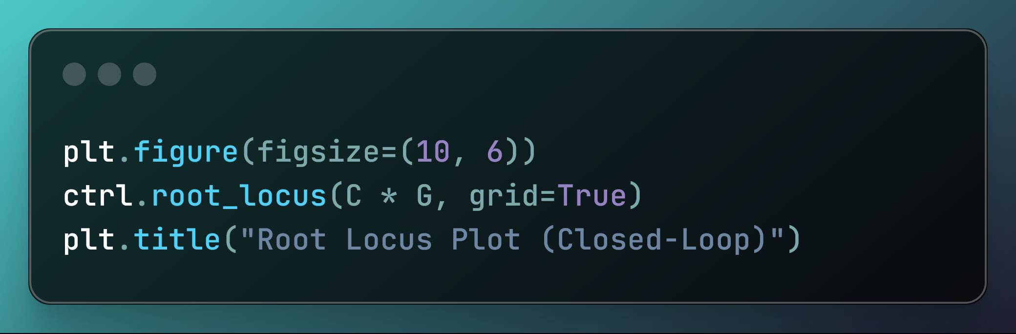 Create the Root Locus Graph
We generate this plot:
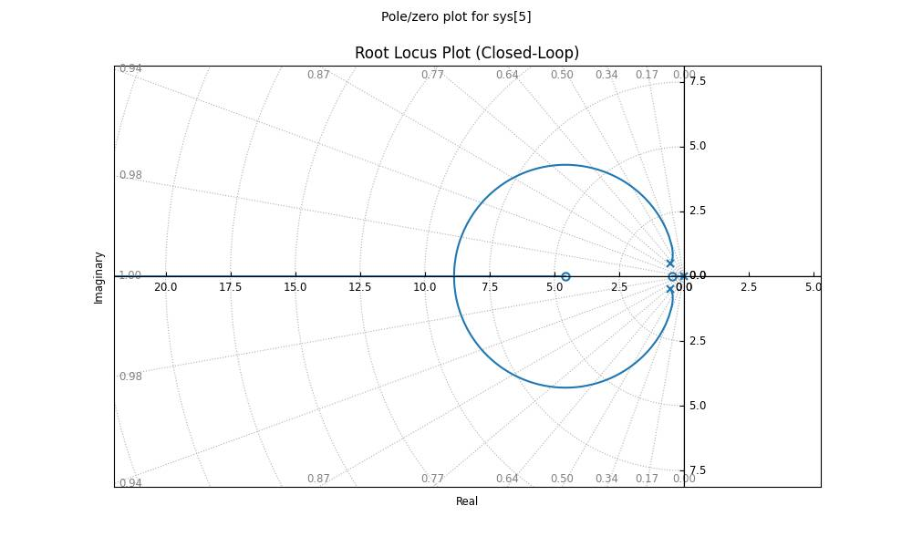 Simple Root Locus Graph
This is a root locus graph. It was invented to help engineers study the stability of control systems.
The crosses on the graph, called poles, are very important.
If they are on the left side of the graph, the system is stable. If they are on the right side, the system is unstable.
The more to the left they are, the quicker the system will return to normal after a disturbance, and thus, the more stable it will be.
But moving more to the left can cause too many oscillations, depending on their specific locations.
The key point is:
- By changing the
Kp,Ki, andKd, this moves the poles to be as far left as possible without causing oscillations.
However, the root locus graph is not enough to ensure stability. We need to use the Bode and Nyquist plots as well. Only with them can we get the best PID controller values for the rocket control system.
Step 6: Bode Plot for Stability Analysis
In this code:
plt.figure(figsize=(10, 6))ctrl.bode_plot(CL, dB=True, Hz=False, deg=True)plt.suptitle("Bode Plot (Closed-Loop)", fontsize=16)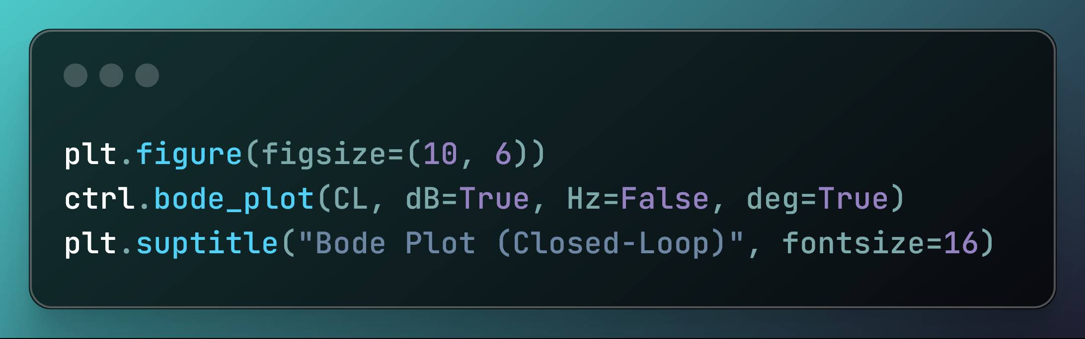 Create the Bode Plot Graph
We generate this plot:
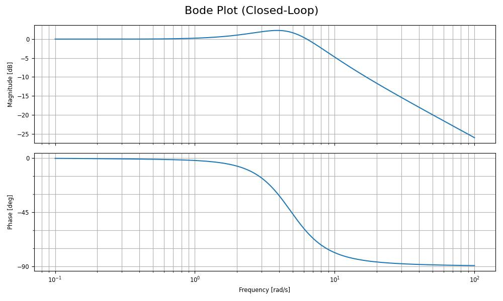 Simple Bode Plot
The Bode plot was invented to help engineers understand how a system responds to changes and how stable it will be under different conditions.
The Bode plot also shows the system’s stability and safety margins.
Let’s understand how it works:
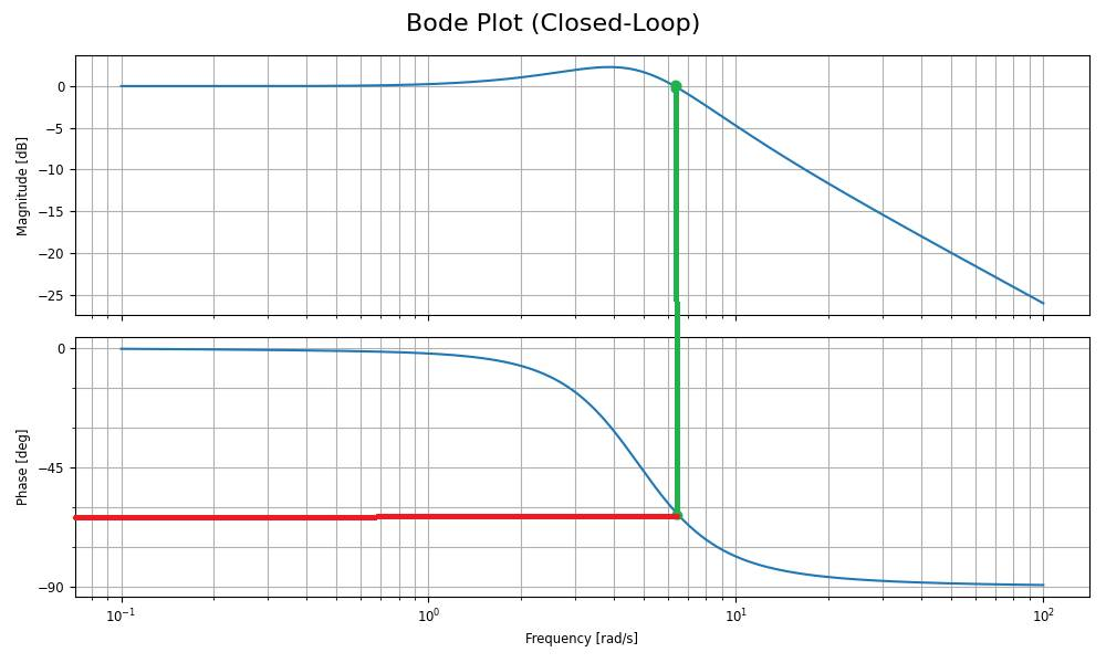 Bode Plot in detail
The graph on top is called the Magnitude Plot and the one below it is called the Phase Plot.
The magnitude plot measures the gain of a system across different frequencies. Higher gain means quicker and stronger reactions, which is good for precise control.
The phase plot measures the phase shift introduced by the system across different frequencies. The phase shift is seen when the gain is 0.
In this case, we can see with the green line when the gain is zero and what phase shift is associated with that in the red line. It is approximately 63 degrees.
An ideal range is a phase shift of 30 to 60 degrees, which balances stability and response speed.
Over 60 degrees, the system is very stable, but might slow down the system response to changes.
So after analyzing the plot, we can conclude this PID controller is stable.
Step 7: Nyquist Plot for Stability Analysis
In this code:
plt.figure(figsize=(10, 6))ctrl.nyquist_plot(CL)plt.title("Nyquist Plot (Closed-Loop)")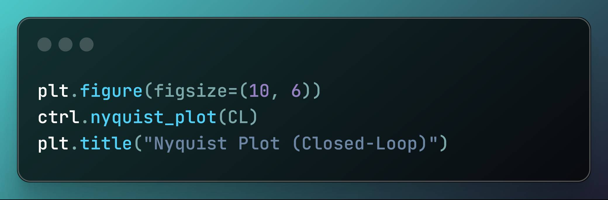 Create the Nyquist Plot Graph
We generate this plot:
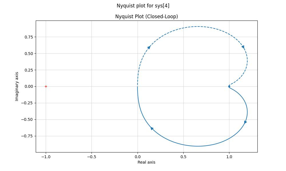 Nyquist Plot Graph
The Nyquist Plot is a tool to help engineers quickly check if a control system is stable or not.
It is very simple:
- If there is no circle around the red cross at point (-1 0), the system is stable.
- If there are circles around the red cross, namely clockwise circles, at point (-1 0), the system is unstable.
Since there aren’t circles around the red cross, this control system is stable.
Last step after designing the rocket control system
After completing the design of this PID control system, we can use tools like Simulink to find the necessary values for many components.
In other words, after getting the best PID controller variables, it’s time to find the physical component values of the rocket.
Some of these values are:
- Resistor values for controlling current flow
- Capacitor values for energy storage
- Inductor values for managing electromagnetic interference
- Sensor calibration values for accurate data measurement and feedback
- Strength and durability of materials for the rocket’s body and fins
- Torque and speed requirements for servo motors
- Spring constants for shock absorption systems
- Pressure ratings for fuel and oxidizer tanks
Thanks to Simulink, we can get all these values needed to design a rocket according to its mission.
With a stable control system, based on a PID controller to control the physical transfer function of a rocket, we can get all the values needed for each component.
Conclusion: Non-linear control systems
 Photo by Peter de Vink: https://www.pexels.com/photo/photo-of-full-moon-975012/
There are many methods available to us to optimize a Linear Time-Invariant (LTI) control system:
- Root Locus Method: Adjust system poles to reduce oscillations.
- Bode Plot Analysis: Maintain phase margin and stability.
- Nyquist Plot: Confirm overall system stability.
With these tools, it’s possible to create a control system.
However, in this process, it is good practice to use methods like the Ziegler-Nichols method to more quickly find the best PID controller variables.
In our exploration, we worked with a very simple rocket system.
In real life, only non-linear tools are used because all rocket systems are non-linear systems.
One example is adaptive control, where the control system adjusts itself in real-time to handle changing conditions
Another one is Lyapunov’s method. In this case, it is used for stability analysis instead of these three plots.
Still, the process of making these control systems is always the same. This article explained how this process works and how it is applied in a time-invariant system.